Simulating Quantum Field Dynamics in 4D Curved Space: Where Quantum Computers Come In
November 7, 2025Introduction
Have you ever wondered how we manage to understand and visualize the fundamental principles of our universe? Much of what we know about the behaviour of physical systems comes from simulations – mathematical and computational models that let us explore phenomena beyond direct experimentation.
For example, we know that particles emerge from their underlying fields, like a photon from an electromagnetic (EM) field. But what if we could understand how these fundamental fields behave in extreme conditions, like when 4D spacetime curves or stretches? Simulating quantum fields in such conditions would enable our understanding of their behaviour during the first moments of the Big Bang and in regions around black holes. We would also be able to make or improve our predictions of the development of physical systems in our universe.
Some aspects of these systems can be simulated with classical computers. However, as the complexity of simulations grows exponentially, classical computers reach their limits and struggle to handle the growing computational demands. In the prospective future, simulations will be done with a new generation of computers – quantum computers.
This article will explore how digital quantum computing can be used to simulate the behaviour of quantum fields under conditions of space curvature in 4-dimensional space, and why this represents the next major step in our understanding of the universe.
Content
Background
Quantum Fields and Vacuum Fluctuations
Classical Simulations
The Problem: Exponentially Growing Information
Simulating Quantum Field Fluctuations in Curved 4D Spacetime with Quantum Computing
Approaches to Simulation
Digital Quantum Simulation Methodology for Curved-Spacetime Fields
Discretizing Spacetime and the Field
Encoding the Degrees of Freedom into Qubits
Hybrid and Advanced Techniques
The Current Problem with Digital Quantum Simulations
Quantum Progress
Why Do Simulations of Quantum Field Dynamics Matter?
Conclusion
About Me
Bibliography
Background
Quantum Fields and Vacuum Fluctuations
In quantum field theory (QFT), particles are localized excitations – quanta – of fundamental fields acting in a Hilbert space. When a field is expanded into spatial modes, each mode behaves like a quantum harmonic oscillator with ground-state energy and vacuum fluctuations.
Vacuum fluctuations arise from the Heisenberg uncertainty principle, which states that position 𝑥 and momentum 𝑝 variables cannot be defined simultaneously with precision for each mode [1]. This principle requires nonzero ground-state fluctuations. Because a continuous field has infinitely many modes, fluctuations are present at every scale – the field fluctuates at each point in space. These fluctuations are always present, even in a vacuum and at absolute zero [2].
Do these vacuum fluctuations show up in everyday life? Yes – theory, observations, and experiments strongly support them. Their effects appear across all scales, from atoms to the cosmos, shaping the universe we observe.
We constantly experience the fluctuations of quantum fields all around us. Several phenomena reveal that the quantum vacuum is not empty. At regular scales, the Casimir effect demonstrates these fluctuations: a force is observed between two parallel conducting plates in a vacuum due to the quantization of the EM field. We also observe fluctuations through the Lamb shift (alterations in an element’s spectral lines) and spontaneous emission from atom-vacuum field interactions. These effects provide direct evidence of quantum field fluctuations.
On larger, cosmic scales, we can see the effect of quantum field fluctuations through the impact of inflation. Inflation stretched quantum fluctuations into regions of slightly higher or lower energy density that became classical density perturbations after inflation – differences in curvature and matter density across space. Their imprint appears as temperature anisotropies in the cosmic microwave background (CMB), and in the known large-scale, cosmic structure: stars, galaxies, and clusters [3].

(Fig. 1)
The 2018 Planck map of the temperature anisotropies of the CMB, extracted using the SMICA method. The gray outline shows the extent of the confidence mask. [July 2018]. European Space Agency (ESA) and the Planck Collaboration.
Quantum fields and their fluctuations support some of the core theories like the Standard Model (including QED) and inflationary cosmology. Quantum field fluctuations have been verified to extreme precision in experiments and consistently validated by quantum field equations. QFT and the confirmation of quantum field fluctuations are definitely among the major achievements of modern physics.
Understanding how fundamental fields behave under extreme spacetime curvature – such as near black holes or during the Big Bang – remains one of the greatest challenges in theoretical physics. Simulating quantum fields in curved spacetime could illuminate how the universe behaved in its earliest moments and how particles interact in the most extreme gravitational environments.
Classical Simulations
Classical computers can provide great help with specific tasks in quantum field simulations when QFT becomes analytically intractable. Monte Carlo methods are widely used for static or equilibrium quantities – such as the mass of a proton, dielectric constant, and conductivity [4]. Additionally, tensor networks and other real-time, non-equilibrium approaches target certain dynamic systems.
Monte Carlo (MC) simulations discretize continuous space into a lattice, turning infinitely many field modes into a finite set of variables a classical computer can handle. The computer stores and updates the field values to track how energy moves and interacts. It does this by using an algorithm that samples field configurations according to their path-integral weights and estimates measurable quantities by averaging these weighted samples to approximate expectation values. The expectation values then represent measurable physical quantities – a field’s oscillations, for example.
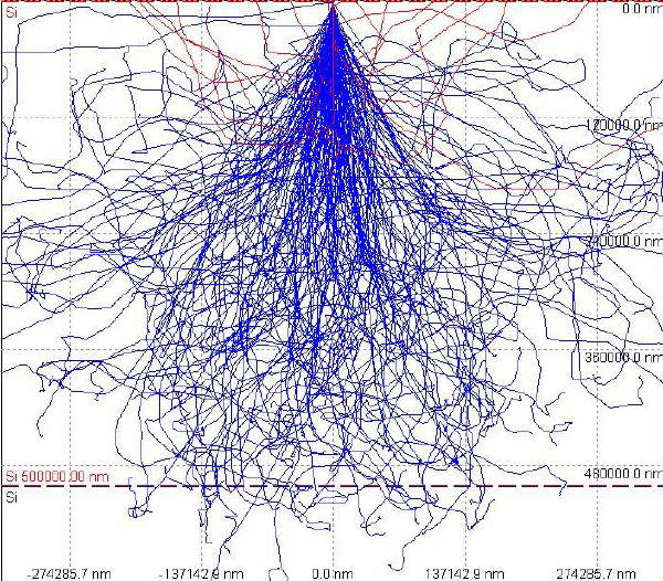
(Fig. 2)
Monte Carlo (CASINO) simulation of possible paths of secondary electrons ionized by a 400 keV Compton electron through a 0.5 mm-thick silicon substrate. When using graphene FETs as radiation detectors, energetic electrons produced by gamma or other ionizing radiation could pass through the substrate and interact with the graphene. [Dec. 2009].
However, MC simulations’ key limitation is their reliance on Euclidean time, established through a Wick rotation, which makes path integrals converge but restricts access to real-time, out-of-equilibrium dynamics. Therefore, MC importance sampling doesn’t work for quantities such as masses of particles (other than light hadrons and nuclei) and quantum chromodynamics (QCD) phase diagrams [5]. In short, MC simulations are best suited to static or equilibrium quantities, while dynamic systems – such as quantum fields evolving during cosmic inflation – remain beyond reach. Other approaches (e.g., tensor networks, Schwinger–Keldysh formalism simulations) can work with real-time behaviour, but they come with their own approximations and errors.
The Problem: Exponentially Growing Information
It is amazing how much progress has been achieved in understanding quantum fields and their nature. Supercomputers extend this understanding by simulating complex physical systems that cannot be understood through quantum field equations alone. However, classical computers face significant computational challenges as system complexity increases.
Discretizing a quantum field on a lattice results in the dimension of the Hilbert space growing exponentially with system size. Simulating a system with real-time evolution requires tracking the full wave function and phase-coherent quantum state – entire superposition and entanglement patterns. Simulating such a system demands memory and computational effort that scale exponentially, making classical simulation intractable.
Fortunately, we can use quantum computers to simulate complex real-time, out-of-equilibrium systems, alongside classical methods. Two types of quantum computing are used: digital and analogue. Digital quantum computing encodes the model in qubits and implements real-time dynamics with gate sequences. Analogue quantum computing uses a controllable system that mimics the target system. Both have advantages: while analogue computing can solve specific problems and is less prone to error, digital computing covers and solves a wider array of problems [6].
In this article, I will focus on digital simulation of quantum field fluctuations, with reference to hybrid and advanced techniques.
Simulating Quantum Field Fluctuations in Curved 4D Space with Quantum Computing
Approaches to Simulation
Simulating quantum field fluctuations in curved or expanding 4D spacetime sits at the intersection of quantum computing and fundamental physics. There are multiple approaches to quantum simulations. Here, I focus on digital, gate-based simulation, optionally paired with classical pre/post-processing or AI-assisted error mitigation. Unlike analogue approaches, digital methods can, in principle, encode a finite discretization of a field with a time dimension, and implement field dynamics via quantum circuits. In what follows, I outline current possibilities for digital simulations of quantum field dynamics in curved spacetime.
Digital Quantum Simulation Methodology for Curved-Spacetime Fields
Digital quantum simulation maps the target field onto a set of qubits and quantum circuits. The key steps include: (i) choosing a finite discretization (spatial lattice or truncated mode basis), (ii) encoding field modes or values into qubits (boson via Fock-space truncation; fermions via standard mappings), and (iii) implementing the field’s Hamiltonian real-time evolution with gate sequences, so that the qubit register mirrors the field’s state and dynamics.
Discretizing Spacetime and the Field
A quantum field with infinitely many degrees of freedom is made finite by either a spatial discretization or mode truncation. The spatial discretization method models continuous space as a discrete lattice. Curvature and expansion are encoded by making the Hamiltonian’s parameters depend on position and time. Therefore, the curved metric of spacetime dictates how the couplings vary, creating a geometry for the field on the lattice.
In the mode truncation method, a finite set of field modes is encoded into qubits. Curvature sets the spectrum and shapes of the modes and their mutual couplings, while the expansion of spacetime makes their frequencies time-dependent. The dynamics of a field are implemented using gate parameters that vary across modes and over time.
Encoding the Degrees of Freedom into Qubits
The next step is to encode the degrees of freedom of a field into qubits. The method depends on whether the target field is bosonic or fermionic.
Each mode of a bosonic field has an infinite Fock space. The space is truncated to a maximum occupation N_max per site/mode, and the occupation number is encoded with a fixed-length code (e.g., binary). Alternatively, boson–qubit mapping can be used to assign basis states (patterns) of qubits to discrete occupation states.
For fermionic fields, occupations are 0/1 per mode/site. Mappings such as Jordan–Wigner or Bravyi–Kitaev translate creation/annihilation operators into qubit Pauli operators, so each mode/site’s occupancy is represented by qubit states. The encoding procedure is independent of the original method for discretization, whether spatial discretization or mode truncation is followed.
Hybrid and Advanced Techniques
Hybrid quantum-classical strategies can aid in executing simulations. Variational quantum simulation could be used to find field ground and vacuum states by using a parameterised quantum circuit (PQC), with adjustable parameters that produce different quantum states and a classical optimiser to minimise an energy function [7].
Additionally, machine learning optimises circuit parameters or formulates encodings. A recent work by RIKEN researchers discovered that stochastic quantization, a method in QFT, parallels the statistical technique of generative diffusion used in deep learning. This approach can significantly speed up lattice field simulations [8].
Another technique is to use photonic continuous-variable quantum computers to simulate quantum fields. Photonic systems (like those developed by Xanadu) manipulate states of light, which are described by continuous variables and can directly represent the modes of a field [9][10].
While these techniques are just at the beginning of their development, they highlight how the wide range of tools can aid and handle quantum field simulations.
The Current Problem with Digital Quantum Simulations
Although digital quantum simulations offer many benefits in simulating quantum field dynamics, there are certain drawbacks to the procedure. Digital quantum simulations are progressing, but today’s hardware remains in the noisy-intermediate-scale quantum (NISQ) stage [11]. Today’s quantum computers typically have 10 – 100 qubits. Factors such as high error rates and low coherence times limit the possible number of operations to roughly a few hundred [12]. To have more error-free operations, error correction and higher qubit counts are required. And simulating quantum field dynamics – especially in curved or expanding 4D spacetime – requires millions of error-free operations. Moreover, the limited qubit count and low coherence time restrict the number of degrees of freedom of a field we can represent and how long we can simulate their evolution before noise overwhelms the signal.
If quantum computers could operate correctly even in the presence of errors [13], we would be able to increase the number of qubits and simulate complex systems more efficiently. Such computers are called fault-tolerant quantum computers—an aim of multiple companies in the industry. But currently, the absence of fault tolerance is the core issue of quantum simulations. In principle, the quantum error correction (QEC) approach can stabilise long computations, but it requires many physical qubits per logical qubit, along with fast decoders [14]. In the case of 3+1D field simulations, thousands to millions of high-quality qubits are needed—an enormous amount.
Recent error-correction milestones are encouraging, and companies like PsiQuantum are rushing to scale up qubit counts through innovative architectures and solutions [15][16]. But currently, the devices remain too small and noisy to run large field models. Simulating complex systems significantly increases depth and sampling costs. In summary, NISQ devices can simulate smaller systems, but simulations of quantum fields in curved 4D space await error-corrected hardware.
Quantum Progress
Fortunately, quantum hardware gradually advances, and in the future, we will be able to simulate complex physical systems efficiently with quantum processors. Recent scientific research also demonstrates important milestones in quantum computing and simulations.
In a recent research paper, researchers simulated the creation of cosmological particles in expanding spacetime with IBM quantum computers. They encoded two bosonic field modes using four qubits, with one quantum of excitation in each mode. Each qubit corresponded to a specific field excitation configuration [17]. This is a clear demonstration of the capabilities of quantum computers in simulating fields in expanding spacetime.
Companies like IBM and Google Quantum AI are working on realising error-corrected quantum computing and have already demonstrated improvements in qubit counts and error rates. For example, IBM’s recent innovations include a superconducting Condor processor with 1,121 qubits and the high-performance Heron processor [18][19]. Both processors expand the scale and improve the error correction of quantum hardware (2023).
The recent improvement of Google’s high-performance quantum chip, Willow, enabled the “first-ever demonstration of verifiable quantum advantage” through the execution of complex Quantum Echoes algorithms [20][21].
These advancements in quantum hardware will enhance the complexity and rate of solving tasks. They will also unlock more practical applications for simulations in different areas, including materials science, drug discovery, and even wider simulations of quantum field dynamics.
(Fig. 3)
Google Quantum AI’s Willow superconducting quantum chip – demonstrated the first-ever verifiable quantum advantage by running the Quantum Echoes algorithm on a 105-qubit array. [October 22, 2025].
Why Do Simulations of Quantum Field Dynamics Matter?
Simulations play a fundamental role in advancing our understanding of physics. Specifically, simulating quantum field dynamics with quantum computing opens a range of pathways through which we can understand physical phenomena and their effects better. Not only do simulations deepen our understanding, but they also let us predict how systems will evolve over time and test these predictions. We can test and formulate theories by simulating quantum field dynamics, as they form the basis of the fundamental theories of physics.
One of the main applications is to better understand early-universe particle production. Simulating the evolution of quantum field fluctuations in expanding or curved spacetime enables our understanding of how particles are created. Running the model of a quantum field backwards to the early moments of the Big Bang would help us reconstruct the creation of particles and plausible past states.
What about theories? Scientists can test a theory by encoding models and checking whether simulated outcomes match the theory’s predictions. This is especially useful where real experiments are impossible. This approach can explain information flow and entanglement near black-hole horizons, a very interesting application.
Simulations can also reveal specific patterns in theories. They demonstrate which terms and variables matter, what can be ignored, and which approximations hold up. These insights can be used to refine models and propose new descriptions.
On the practical side, structured QFT problems can act as a test for a computer. Simulations can help compare algorithms and hardware and identify what scales are feasible now.
Conclusion
Simulating quantum field fluctuations in curved spacetime and understanding their behaviour under extreme gravitational conditions remains a significant challenge.
Despite current hardware limitations, the rapid pace of progress in quantum computations suggests that large-scale simulations may soon be achievable.
When that happens, simulating quantum field dynamics in curved 4D spacetime would allow us to study their nature and effects and understand their behaviour better. Perhaps these simulations will let us extrapolate to more complex cases in physics, and let us uncover some of the fundamental, persisting questions about our universe and existence.
About Me
My name is Veronika Batishcheva, I am a grade 11 student passionate about science and our world. I have an interest in physics (particularly modern physics) and quantum computing. I enjoy learning about quantum computing and other emerging technologies. I also love to extrapolate from physics to quantum computing. Apart from that, I enjoy reading about physics and technology, and I’m always open to learning new things!
Bibliography
Figures
Fig. 1 – Planck 2018 SMICA map of the Cosmic Microwave Background. ESA Planck Picture Gallery, 2018, https://www.cosmos.esa.int/web/planck/picture-gallery
Fig. 2 – Childres, Isaac, Romaneh Jalilian, Michael Foxe, and Yong P. Chen. “Effect of Energetic Electron Irradiation on Graphene — Figure 2.” AIP Conference Proceedings (AIP), 2 Dec. 2009, https://www.researchgate.net/figure/Monte-Carlo-using-CASINO-simulation-of-possible-paths-of-secondary-electrons-ionized-by_fig2_237509571
Fig. 3 – Neven, Hartmut, and Vadim Smelyanskiy. “Our Quantum Echoes Algorithm Is a Big Step toward Real-World Applications for Quantum Computing.” The Keyword (Google), 22 Oct. 2025, https://blog.google/technology/research/quantum-echoes-willow-verifiable-quantum-advantage/
Sources
[1] California Institute of Technology. “What Is the Uncertainty Principle and Why Is It Important?” Caltech Science Exchange, n.d., https://scienceexchange.caltech.edu/topics/quantum-science-explained/uncertainty-principle
[2] Bhaumik, Mani L. “The Enigmas of Fluctuations of the Universal Quantum Fields.” arXiv, 11 Dec. 2023, https://arxiv.org/abs/2401.08638
[3] Agulló, Iván, José Navarro-Salas, Gonzalo J. Olmo, and Leonard Parker. “Inflation, Quantum Fields, and CMB Anisotropies.” General Relativity and Gravitation (Springer), 2011, https://s3.cern.ch/inspire-prod-files-e/eb435c2e60233137c03e5f6387c8ae83.
[4] Wang, Yazhen. “Quantum Monte Carlo Simulation.” The Annals of Applied Statistics (Institute of Mathematical Statistics), June 2011, https://www.jstor.org/stable/23024900.
[5] CERN Quantum Technology Initiative. “Hybrid Quantum Computing Infrastructures, Algorithms and Applications.” CERN, n.d., https://quantum.cern/quantum-computing-and-algorithms
[6] Pasqal. “Analog and Digital in Quantum Computing.” Pasqal (Pasqal), n.d., https://www.pasqal.com/analog-and-digital-in-quantum-computing/.
[7] McArdle, Sam, et al. “Variational Ansatz-Based Quantum Simulation of Imaginary Time Evolution.” npj Quantum Information, vol. 5, 2019, https://www.nature.com/articles/s41534-019-0187-2
[8] Wang, Lei, Gert Aarts, and Kai Zhou. “Diffusion Models as Stochastic Quantization in Lattice Field Theory.” Journal of High Energy Physics, vol. 2024, no. 5, 2024, article 060, https://link.springer.com/article/10.1007/JHEP05(2024)060
[9] Xanadu. “Photonics.” Xanadu, n.d., https://www.xanadu.ai/photonics/
[10] “Scaling and Networking a Modular Photonic Quantum Computer.” Nature, 22 Jan. 2025, https://www.nature.com/articles/s41586-024-08406-9
[11] Leyton. “Quantum Computing: Vision and Challenges.” Leyton Canada, 28 May 2025, https://leyton.com/ca/insights/articles/quantum-computing-vision-and-challenges/
[12] Funcke, Lena, Tobias Hartung, Karl Jansen, and Stefan Kühn. “Review on Quantum Computing for Lattice Field Theory.” arXiv, 1 Feb. 2023, https://arxiv.org/abs/2302.00467
[13] Davis, Robert, Olivia Lanes, and John Watrous. “What Is Fault-Tolerant Quantum Computing?” IBM Quantum Computing Blog, 30 May 2025 https://www.ibm.com/quantum/blog/what-is-ftqc
[14] QuEra Computing. “Quantum Error Correction.” QuEra, n.d., https://www.quera.com/glossary/quantum-error-correction
[15] “PsiQuantum Plans Quantum Supercomputer That Runs on Light” IEEE Spectrum, n.d., 5 Oct. 2025 https://spectrum.ieee.org/psiquantum-supercomputer
[16] PsiQuantum. “Building the Future of Computing.” PsiQuantum, n.d., https://www.psiquantum.com/
[17] Maceda, Marco D., and Carlos Sabín. “Digital Quantum Simulation of Cosmological Particle Creation with IBM Quantum Computers.” arXiv, 3 Oct. 2024, https://arxiv.org/abs/2410.02412
[18] Gambetta, Jay. “The Hardware and Software for the Era of Quantum Utility Is Here.” IBM Quantum Blog, 4 Dec. 2023, https://www.ibm.com/quantum/blog/quantum-roadmap-2033
[19] IBM Quantum. “Technology for the Quantum Future.” IBM, n.d., https://www.ibm.com/quantum/technology
[20] Chen, Yu, and Michel Devoret. “Our Quantum Hardware: The Engine for Verifiable Quantum Advantage.” The Keyword (Google), 22 Oct. 2025, https://blog.google/technology/research/quantum-hardware-verifiable-advantage/
[21] Neven, Hartmut, and Vadim Smelyanskiy. “Our Quantum Echoes Algorithm Is a Big Step toward Real-World Applications for Quantum Computing.” The Keyword (Google), 22 Oct. 2025, https://blog.google/technology/research/quantum-echoes-willow-verifiable-quantum-advantage/